The Tolman-Eichenbaum Machine
Cognition as Spatial Manipulation

Spatial considerations are hard-wired into how the brain processes information, yet frontier AI models mostly leave space to be learned implicitly from data. Evidence from neuroscience suggests that the spatial machinery of the brain is involved in far more than just navigating space. The hippocampus, which is evolutionarily responsible for mapping space among all invertebrates from fish to humans, is also involved in relational memory, reasoning about social hierarchies, and even high-level problem solving. So then why do modern AI models ignore spatial representations, when they potentially play a critical role in human reasoning and cognition? Perhaps a better understanding of spatial reasoning in the brain could help us to build more powerful thinking machines. I’ve previously discussed at length in this blog how the brain has not one, but two separate mechanisms for processing space (one allocentric and the other egocentric), and that these mechanisms of what and where can also be hijacked for abstract thinking. In this article, I examine the Tolman Eichenbaum Machine (TEM) by James Whittington et al., a trainable artificial hippocampus that experimentally replicates biological features such as grid, border, band, and place cells while providing an explicit computational account of how spatial reasoning can be performed in the brain.
Motivational Principles
The TEM is named after Edward Tolman, who discovered the role of the hippocampus in navigation, and Howard Eichenbaum, who established its use in cognitive and social reasoning. It is trained with simulations and example problems to predict the next sensory input given prior sensory inputs, much as LLMs are trained to predict the next word given prior words. Thus, any spatial reasoning the TEM learns is inferred to explain the sensory data. The purpose of the TEM is to demonstrate that the same computational structure can simultaneously represent navigation, memory, and basic symbolic reasoning.
The TEM is built on the following principles:
Space is a graph of actions. That is, you know space because of how you move through it. Space consists of places you can be and ways can move between them. Each place is a node in the graph, and each movement takes you from one node to another. From the perspective of the hippocampus, every action is a movement, and hence space is a collection of places connected by actions. See Figure 1(C) below for an example; it shows four places, and four actions to move between them: NORTH, SOUTH, EAST, WEST.
Sensory inputs are objects that must be placed on the graph. One of the main characteristics of space is that it can be filled by different objects at different times. So, for example, if you are at home you will have one map of the space around you, and at the office you will have a different map. In each case, space behaves the same, but the objects occupying that space are different.
Logical relations can be laid out as actions on a spatial graph. In Figure 1(A), we see that family relationships can be determined from a spatial representation. In this case, we imagine the family roles as places that are filled by people. Then, we can treat family relationships as movement in this family space. Logical relationships are nicely maintained by this analogy; for example, mother and daughter are inverse relationships simply by the fact that they move in opposite directions. As Figure 1(C) shows, the logic of transitive relationships also works well with spatial representations.
Short-term associations between space and objects must be learned quickly. The usefulness of representing space is that it behaves the same across many tasks. But to use space, you have to know what is in it, and the contents of space must be relearned every time you go to a new place. Thus, the TEM distinguishes between a long-term model of spatial behavior, which it learns through backprop, and a short-term memory of spatial contents, which is modeled as a Hopfield network with local Hebbian updates.
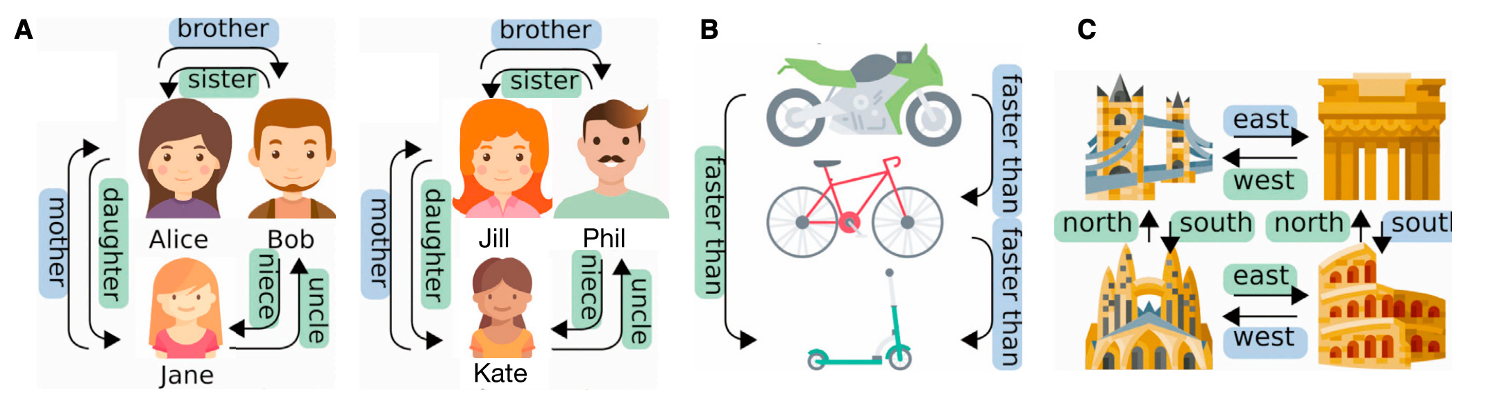
Figure 1 from the TEM paper: illustrating spatial relationships (Whittington et al, 2020)
It is worthwhile to step back and consider some of the advantages of building on the principles above. Firstly, navigation tasks can be solved in this framework: if you know where in space you wish to go, then you can find a sequence of actions that will take you there. Secondly, basic logical reasoning can also be solved in the same framework by the same method. To answer the question “Who is Alice’s brother”, we need only locate Alice in pseudo-space, and then take the brother action to find Bob. Thirdly, we can reuse the same planning and representational framework for navigating or reasoning in many different contexts; our long-term knowledge of how space works transcends the particular tasks being solved at any given moment.
Algorithmic Design
The purpose of the TEM is to infer position in space and to associate objects to positions in space on a temporary basis. These inferences are driven by two inputs: the sequence x_t of sensory observations and the sequence a_t of actions at each time step t. The inferred hidden states are the position in space, g_t, and the association p_t which represents the pair (x_t, g_t) associating the object observed at time t to its position at time t. The variable names are chosen so that g_t represents the firing of a grid cell, and p_t represents the firing of a place cell.
Notably, the authors made the sensory inputs and actions categorical, starting with one-hot vector representations (d=45). Then they compressed these one-hot representations into a 10-dimensional representation in such a way that the resulting vectors used a two-hot representation, for a sparsity factor of 20%. The choice to use so few dimensions is needed in the original architecture, but a later transformer implementation removes some of the need for low dimensions.
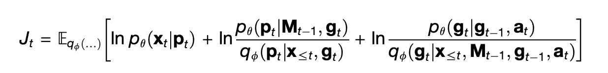
The TEM is designed as a conditional probabilistic model, that is, as a joint probability distribution p_θ over x_t, g_t, and p_t given a_t computed by a series of neural networks parameterized by a set of variables θ. From the paper:
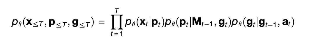
The factorization into three terms on the right is what allows TEM to separate space from content. The term p_θ(g_t | g_{t-1}, a_t) means that the current position g_t is guessed by finding the previous position g_{t-1} and then moving according to the action a_t. Then the term p_θ(p_t | M_t, g_t) guesses the pair p_t at current position by looking in the memory M_t at position g_t. Finally, p_θ(x_t | p_t) guesses the expected sensory percept given what was retrieved from memory, based on the simple heuristic that a place in space is probably still occupied by what ever you saw there last.
The model p_θ allows us to run the model and predict the sensory input x_t from the previous position g_{t-1}, the action a_t, and the memory contents M_t, but we don’t have the previous position g_{t-1} yet!
To fill this gap, the TEM is defined as a variational auto-encoder (VAE). A VAE has two parts: an encoder that converts its input into a proposed hidden state of the world, and a decoder that attempts to reproduce the input from the from the hidden state. The encoder and decoder are both joint probability distributions over the input and the hidden state, each parameterized by separate neural networks. The model p_θ is the generative decoder, but we have not defined the encoder for inference that will tell us the position of an object based on sensory input and actions.
The reason for having two models is due to classical quirk of statistical models. In statistical models, inference (the encoder) and generation (the decoder) are two sides of the same coin; the math tells you how to solve one given the other. However, for almost every powerful model, if inference is computationally tractable (inference), then the decoder (generation) is usually intractable and vice versa. Variational methods thread this needle by designing not one, but two independent models — one model (the encoder) that is tractable for inference, and another (the decoder) that is tractable for generation. Then both models are trained to be as similar as possible, that is, to model the same ultimate joint distribution after training, using a loss criterion called the evidence lower-bound (ELBO).
In the case of the TEM, the (inference) encoder is another model qᵩ defined as
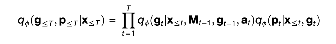
In this model, the right-hand side has two terms. The first term looks up a proposed association ^p_t from the prior memory M_{t-1} given the sensory input x_t, and then uses a neural network to extract the expected position g_t from the proposed association, the prior position g_{t-1}, and the action a_t. The second term then combines the new position g_t with the sensory input x_t to yield the final association p_t. Then, the memory M_t is updated with the new association p_t.
The full inference and generation process is shown in Figure S3 from the paper.
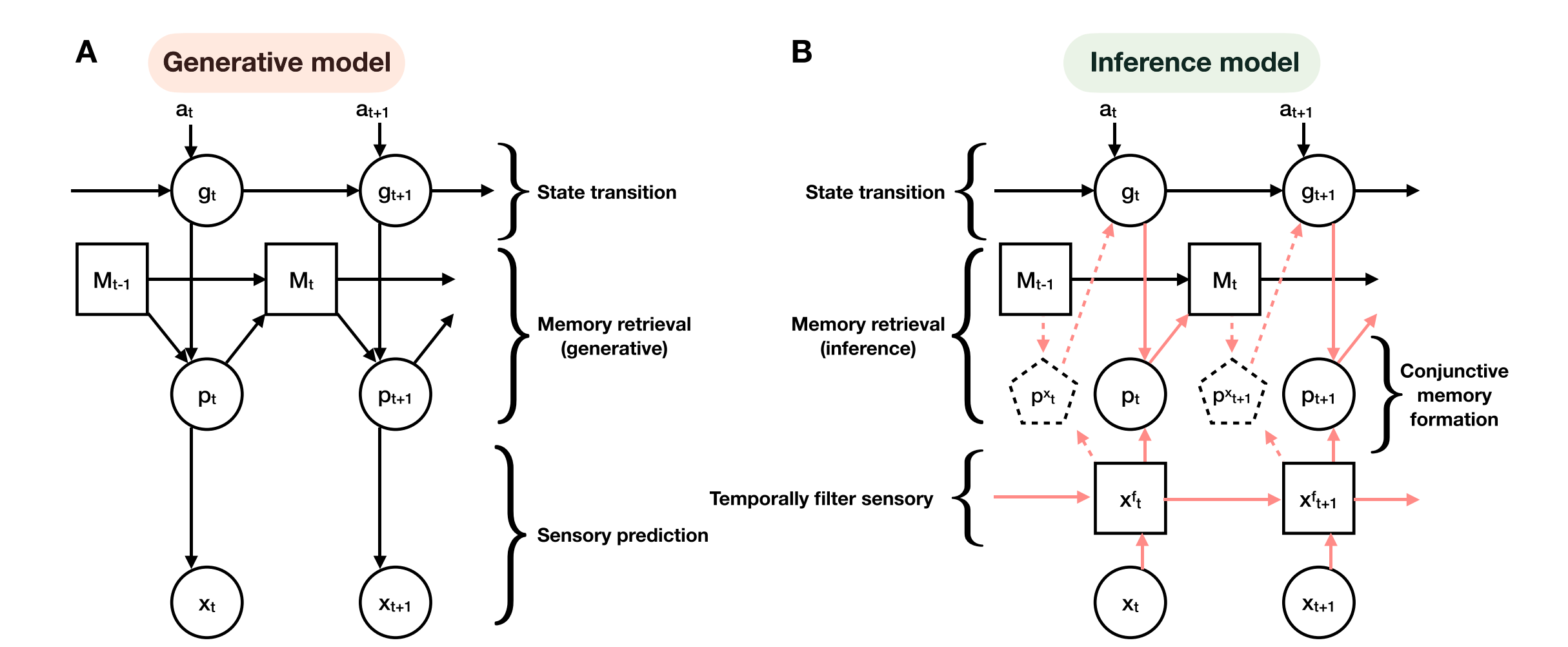
Figure S2 from the TEM paper: block diagram of the model (Whittington et al, 2020)
The VAE described above, except for the memory M_t, is trained using backprop with the ELBO loss on p_θ and qᵩ:
So then what about the memory? Whereas the current state of AI provides a standard methodology for training the model p_θ, there is no standard notion of an associative memory. The authors of the TEM paper choose a Hopfield network, which is an older model of memory. The advantage of this choice is that it rapidly updates content as

This memory retains content much faster than backprop, and hence serves as a suitable short-term association between space and its contents. The disadvantages of this choice center the nature of p_t in the original TEM paper.
Thus the authors set p_t as the flattened vector representation of the outer product P_t of the senses x_t and the position g_t, so that P_t = g_t x_t^T. This design choice has some significant downsides, chiefly that the dimension of p_t is the square of the dimensions of g_t and x_t. But it also means that the contents p_t can be looked up either from the position g_t or the sensory input x_t, which is crucial to the algorithm above. The lookup uses a recursive fixed-point search attributed to Ba et al. (2016):

where h_0 is variously x_t or g_t as required.
It is worth mentioning that the representation of P_t implies that x_t and probably g_t are sparse vectors. Otherwise, the memory capacity of M_t would be significantly reduced. Notably, Whittington et al. used two-hot categorical vectors for x_t, yielding the needed sparsity for this approach.
In a follow-on paper, Whittington et al. (2022) realized that the memory could be represented as the hidden layer of a transformer attention based on Ramsauer et al.’s recognition that these hidden layers implement a Hopfield network, and they published the TEM-t variant of the TEM model built around this idea. I actually think there’s a better way to map TEM onto transformers, and I’ll cover that in a future post (cf. this post for background). However, it’s worth mentioning now that TEM-t encodes TEM into a transformer by overriding the positional embedding to reflect the position g_t. By doing so, the positional embedding in the transformer becomes dynamic and dependent on the action a_t, which should make the transformer much more versatile, although the implementation in TEM-t breaks the computationally parallel design of the transformer.
Overall, however, the design of the TEM suitably implements the principles for which it was designed and can be trained just from the task of predicting the next sensory input.
Training TEM
Recall that the goal of the TEM is to demonstrate that the same spatial representation can simultaneously model basic tasks of navigation, memory, and cognition. Thus the TEM was trained in simulations of movement through a variety of small synthetic worlds.
In a simulation, the world is a graph whose nodes are connected by actions. The simulation worlds are synthetically generated from four types of tasks:
Transivitive Inference. A set of 4-6 objects are placed in a line, with each object serving as a graph node, e.g. apple, pear, monkey, diamond. The action space has two parameters: the direction higher or lower, and the number of steps to move on the line. The learned space can then be trained to answer questions such as “Does pear come before diamond?”
Social Hierarchy. A family tree of depth 3 or 4 and branching factor two (each parent has two children) is populated with an arbitrary set of names. Gender is removed for simplicity, and the action space consists of 10 relationships such as sibling, parent, grandparent, child 1, etc. The learned space should be able to answer questions such as “Is Bob one of Suzie’s grandchildren?”
Graph Navigation. A range of 2-D graphs is instantiated with either as a rectangular grid of width 8-11 or as a hexagonal grid of width 5-7. In general, grid cells in mammals use a hexagonal pattern. Presumably (the authors do not clarify) each node of the grid is given assigned a unique one-hot label used to identify the node. The action space (also presumably) consists of moving to neighboring nodes on the grid, i.e., 4 actions (N, E, S, W) on a rectangular grid and 6 actions on a hexagonal one. This tasks mimics the navigation capabilities of the hippocampus.
Loop tracks. The purpose here is to simulate a case in which rats run around a circular track, but only receive a reward on the 4th time through a track of length 8. For an unknown reason, the authors modeled this as a graph with 32 nodes (4 loops of 8 steps) instead of the more obvious 8 step loop (an octagon), and the action steps are presumably backward and forward around the loop. This task is intended to represent non-spatial navigation, though it seems very spatial to me.
In a simulation, an agent is placed at a node in the graph, and then navigates the graph according to an action plan generated a priori as part of the data. The authors generate two kinds of action plans for use in training: random movement that traverses a random edge at each step for all tasks, and behaviorally directed movement that prefers exploring novel stimuli for half of the graph navigation simulations. These novel stimuli are modeled by marking certain nodes as “shiny” and biasing movement to favor shiny nodes.
At the beginning of a simulation, two separate memory modules M_t are initialized to be blank, one for the decoder and one for the encoder. The simulation is then run for many steps (2k-5k for graph navigation, less for the others).
In order to represent multiple time scales and hierarchical learning, the authors used temporal smoothing to generate 5 different sensory input sequences from the data in each simulation, with one being the base-level sensory input, and the other four progressively averaging over longer time frames to make shorter and shorter input sequences. Each simulation was then run at each of these time scales.
The dimension of g_t varied based on the time scale from 30 on the base input down to 18 for the highest scale; these were dimensionally reduced to 10 (resp. 6) to generate the association p_t; combined with the 10-dimensional sensory input, this resulted in a dimension of 100 down to 60 for p_t.
During training, reading the estimated position g_t from the memory in the encoder qᵩ is initially suppressed by controlling variance of qᵩ(g_t | M_t, x_t) until the TEM learns to use the memory properly.
After training, the TEM is trained to predict the sensory inputs that will result from each action. One can then use the TEM to navigate by choosing actions that will result in a desired input. So, for instance, to answer the question “Who is Bill’s grandmother”, we can provide the TEM with the sensory input x_t=Bill, take the action grandmother, and finally read off the value of x_{t+1} as the answer.
Experimental Results
In evaluating the TEM as a model of the hippocampus + entorhinal system, we can ask the following core questions:
Do the positions g_t actually model space in a meaningful sense?
Do the place associations p_t model spatial content in a meaningful way?
Do the activations and functions of the positions g_t correspond to the experimental data recorded from cells in the mammalian entorhinal cortex?
Do the activations and functions of the place associations p_t correspond to the experimental behavior of hippocampal place cells?
In discussing the results, keep in mind that the positions g_t are intended to model grid cells in the medial entorhinal cortex, and the place associations p_t model place cells in the hippocampus. As an aside, sensory input x_t is meant to correspond to the lateral entorhinal cortex.
TEM grid cells model spatial position. Given a sequence of actions that start and end at the same position (e.g., N → E → S → W in cardinal directions as a_1, a_2, a_3, a_4), the trained TEM infers the same position for the start and end steps (i.e., g_1 = g_4). Thus for a given synthetic graph world, we can talk about the position of a node a as g_a, independent of when it was visited. Furthermore, TEM learns different representations for each node, so that for distinct nodes a and b, we have g_a ≠ g_b. These representations are also peaked in the activation landscape, meaning that different positions are distinct from each other and well-separated. Also, for the graph navigation worlds, distance between nodes in the graph is reflected in the TEM position representations, so that g_a and g_b are more different the further they are from each other. Finally, these positions are reused across tasks; if there is a cluster of activations at a position g in one environment, that same cluster tends to be used as a representation of a position in other environments as well.
TEM place cells represent content at particular positions. The place cells p_t are strongly correlated with specific g_t across environments. Thus, given a node position g_a, there are several corresponding place cells p_a^1, p_a^2, etc. that represent the present of a task-specific object at position g_a, and these relationships are stable across tasks, with only the object content differing. So the place associations p_t really do reflect (object, position) pairs.
TEM can answer questions about logical and spatial relationships. After training, a new synthetic world can be generated, and by traversing each node in this world once, TEM can answer questions of various kinds, including:
Social hierarchy: “Who is Joe’s aunt” can be answered by inferring the position g_1 from x_1= Joe, taking the action a_1=aunt, and inspecting the inferred x_2.
Object positioning: “What object is two spaces to the right of the apple?” in the arrangement apple, pear, monkey, diamond. One infers the position g_1 from x_1=apple, takes the action a_1 =(higher, 2), and reads off x_2=monkey.
TEM representations are similar to mammalian hippocampus recordings of place and grid cells. Figure 4 of the paper, reproduced below, shows generated data in hexagonal and rectangular environments (in rainbow colors) alongside biological data recorded from rats (in black-and-white). Further, the graphs on the bottom right of the figure show significant correlations between activations of TEM vs. rat place cells.
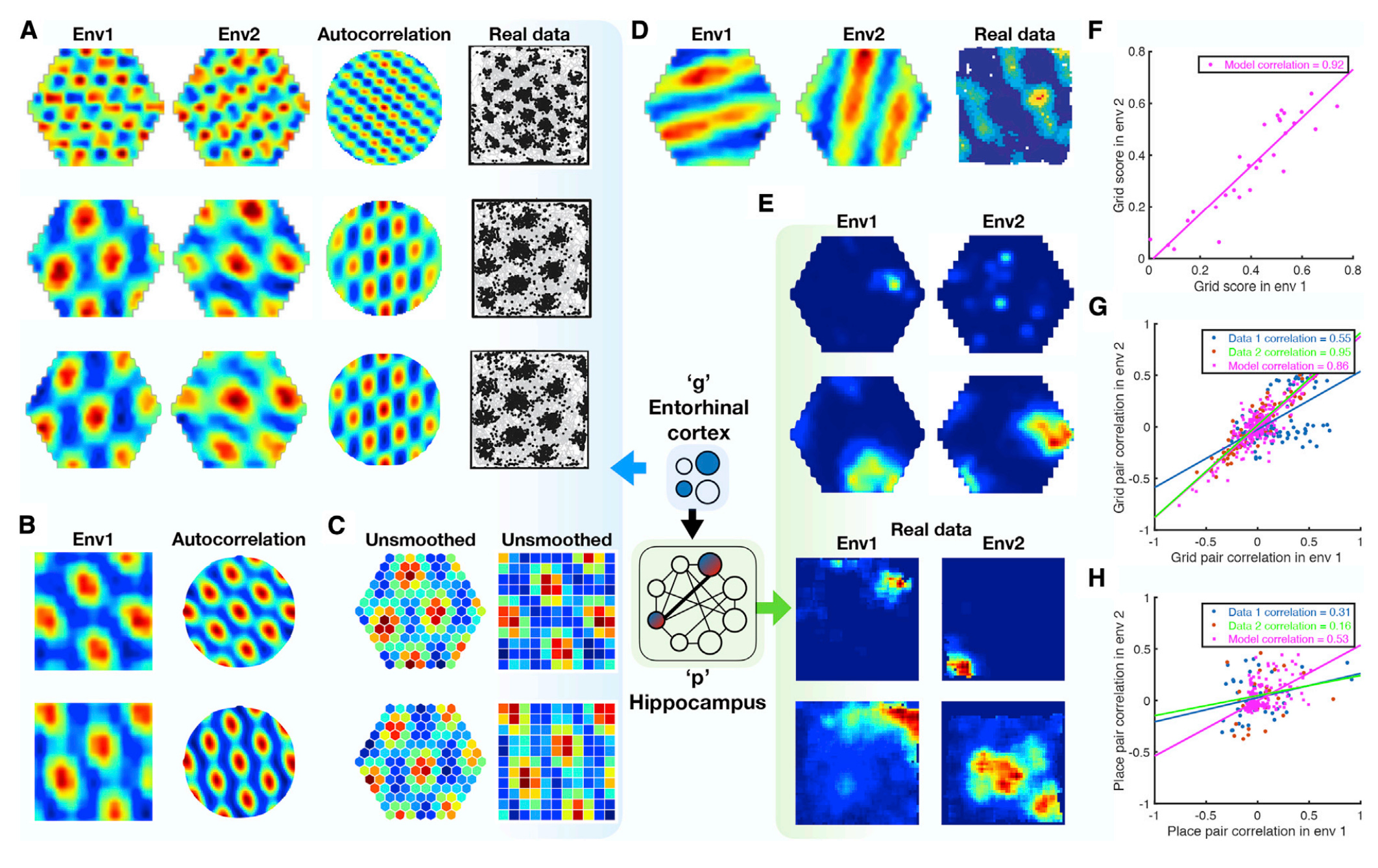
Figure 4 of the paper compares TEM data with biological data (Whittington et al., 2021).
Conclusions
The TEM shows that spatial position can be learned from sensory data, that biological navigational representations can be obtained from training in simulations, and that the same representations can span navigation, memory, and cognition. These observations support the claim that spatial navigation plays a role in the development of higher-order cognition in some way.
Nonetheless, with only 45 categorical inputs and 30-dimensional position representations, the TEM is clearly a toy model. Furthermore, the tasks on which the TEM was trained were highly curated and simplistic. It is not clear how to use the TEM as part of an industrial-scale AI model, nor has its value in practical problem-solving settings been demonstrated.
Most importantly, the TEM cannot tell us how to create plans and assign representations for higher-order problem solving. Where do the sensory input choices come from? How would the brain choose which actions to represent with specific spatial relationships? Why should the brain choose to use spatial representations to solve these problems at all?
Hence, the next question is how we could use the design principles of the TEM as part of a larger system that selects goals, decomposes them into subgoals and subtasks, and executes hierarchical plans, whether for navigation or cognitive problem-solving.
In the next post, I will return to some of the concepts discussed previously in this blog (e.g. here and here) in order to design a research plan that takes advantages of spatial structure like that of TEM in order to learn to plan and reason hierarchically.
Couldn't agree more. Connecting spatial reasoning from neuroscience to AI is realy crucial for building truly intelligent systems. Thanks for this insightful read!